
The Problem
Cyber attacks are bad. And Distributed Denial-of-Service (DDoS) attacks, specifically, can cause financial loss and disrupt critical infrastructure. Sometimes utilizing millions of devices, the effects of these attacks range from stopping stock market trades, to delaying emergency response services. While there are commercial products that monitor individual businesses, there are few (if any) open, global-level, products. Wouldn’t it be great to have a DDoS alerting and reporting system for government and international agencies that:
- Doesn’t require a direct attack on their network, and
- Uses a non-proprietary data source
A Solution
This may be possible with machine learning and Border Gateway Protocol (BGP) messages, and we present a technique to detect DDoS attacks using this routing activity. The ultimate goal is to detect these as they happen (and possibly before)… but baby steps. If we can do this at the day level, it will give some hope that we can do this at smaller time scales. This will bring its own separate challenges, but we save this for the discussion section.
The Data
To obtain data suitable for machine learning (preprocessing), there are a number of steps we take. The general outline is that we use BGP communication messages, bin them by time (10-minute intervals), and then aggregate them by IP range (/24 CIDR block). We extract features during the aggregation producing our starting dataset. To normalize the data points, we use anomaly detection (placing everything in the set {0-normal, 1-anomalous}). This also incorporates the time bins into the dataset. Finally, we use a CIDR block geolocation database to assign country, city, and organization (ASN) information. The resulting dataset is what we use to classify.
Border Gateway Protocol (BGP)
BGP keeps track of Internet routing paths and CIDR block (IP range) ownership by Autonomous Systems (AS’s). AS’s broadcast changes to the paths between CIDR blocks, And due to BGP’s age and ubiquitous use, sensors have been placed at various locations to allow the recording of broadcast traffic. This is used to monitor the health of the Internet as a whole and detect network disruptions when present. Due to this global-scale monitoring, we collect data from two available (and open) BGP message archives and the data is binned by 10-minute intervals. RIPE NCC collects Internet routing data from several locations around the globe, and the University of Oregon’s Route Views project is a tool for Internet operators to obtain real-time BGP information.
The raw data for this experiment is available on Open Science. The data covers over 60 large-scale internet disruptions with BGP messages for the day before and during for the event. Just know that the data is over 200GB before you decide to download it.
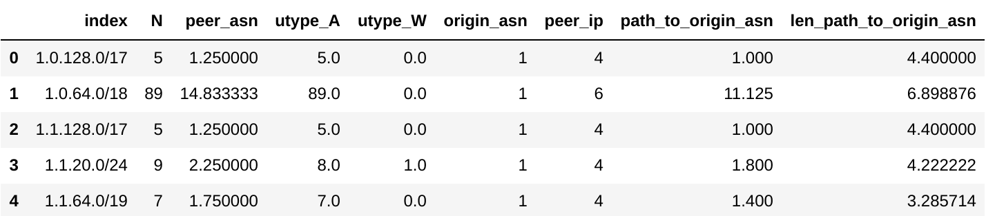
Features & Aggregation
Our entity (or unit-of-analysis) for the raw BGP data consists of /24 CIDR blocks across 10-minute intervals. We record:
| Feature Name | Quick Description | Aggregation |
| Origin CIDR Block | A range of IP addresses | GROUPBY( Origin CIDR Block ) (the entity) |
| Origin AS | the Autonomous System to which the Origin CIDR belongs | COUNT( DISTINCT( Origin AS )) |
| Path to Origin AS | the list of AS’s traversed to arrive at the Origin CIDR | COUNT( DISTINCT( Path to Origin AS )) / COUNT( * ) |
| Path to Origin AS | the list of AS’s traversed to arrive at the Origin CIDR | AVG( LENGTH( Path to Origin AS )) |
| Announcements | the AS path to be set | COUNT( * ) |
| Withdrawals | the AS path to be removed | COUNT( * ) |
| Peer AS | the Autonomous System making the broadcast | COUNT( DISTINCT( Peer IP )) / COUNT( * ) |
| Peer IP | the specific IP making the broadcast | COUNT( DISTINCT( Peer IP )) |
Anomaly Detection with Isolation Forest
At this stage, we have a dataset of aggregated features, binned by 10 minute time intervals. We make the assumption that normalizing the data to highlight potential network disruptions will allow machine learning models to better discriminate. To that end we employ the anomaly detection technique Isolation Forest. Standard transformation/normalization techniques (e.g. min-max scaling) weren’t chosen here, as we needed to take past states/features into consideration as well. Isolation Forest allows for this, as we can “train” using the past states (previous 3 hours) and “predict” on the current 10 minute bin. We (horizontally) stack the results to produces a dataset of shape number-of-CIDRs by 10-min bins, where the values are in {0-normal, 1-anomaly}.
Isolation Forests are a modification of the machine learning framework of Random Forests and Decision Trees. Decision Trees attempt to separate different objects (classes), by splitting features in a tree-like structure until all of the leaves have objects of the same class. Random Forests improve upon this by using, not one, but several different Decision Trees (that together make a forest) and then combines their results together. An Isolation Forest is the anomaly detection version of this, where several Decision Trees keep splitting the data until each leaf has a single point. This algorithm uses “the average number of splits until a point is separated” to determine how anomalous a CIDR block is (the less splits required, the more anomalous).
CIDR Geolocation
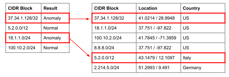
CIDR blocks don’t contain information about their relationship to each other (geographical, relational, or otherwise), but we know some disruptions are related by geography (natural disasters) and organization (Verizon Business). To account for this we attach country, city, and AS information to the CIDR blocks and obtain a dataset of shape entity (country/city/AS) by feature by time. Following this, the features are stacked after this joining, incorporating geographic relationships into the dataset. The geolocation data is collected from MaxMind’s (free) GeoLite2 database. See this [link] for more details.
Labeling the Dataset
We stack feature vectors across the 3 entity types (country/city/AS). All feature vectors for the top 75 countries (determined by the CIDR blocks contained within) are stacked together for each disruption day, forming a feature matrix (instead of vector) of size 1 x 144 x 75 for countries. The same process is performed for cities and AS’s to produce a dataset of 324-by-144-by-75. 324 = 108 * 3 entity-types. 144 = 24 hours * 6 10-minute bins in an hour.
We are interested in DDoS attacks, so we need to gather data for these events. Looking at various news sources, we collected BGP data across 12 Denial-of-Service attacks (36 data points), that ranged from 2012 – 2019.
Experiment
Data & Code
Our data and test script for the results are available on GitHub [here]. Negative examples are collected from several other internet outages/disruptions. Several days where no major disruptions were reported are also collected. We use a random forest model for prediction, and made several pre-processing decisions before prediction. See the evaluation script for more details. We list specifics below.
Balancing the Dataset
Across the trials, it’s worth balancing the dataset used (by sub-sampling). To do this, we employ the code below. This results in a reduced dataset size of 66-by-144-by-75.
data_pos = data_full[data_labels == 1]
data_neg = data_full[data_labels == 0]
np.random.shuffle(data_pos)
np.random.shuffle(data_neg)
min_len = np.min([len(data_pos), len(data_neg)])
X = np.vstack([data_pos[:min_len], data_neg[:min_len]])
y = np.vstack([np.ones((min_len,1)),np.zeros((min_len,1))])
Data Splitting
After balancing the dataset, we make our train/test split. Due to our data transformation scheme (generating 3 examples per cause outage), we take extra care not to poison results by mixing data from the same event in training and test. Due to this splitting requirement, we use the train/test splitting code below.
import numpy as np
from sklearn.model_selection import StratifiedShuffleSplit

index = list(range(0,len(data_full),3))
indices = list(StratifiedShuffleSplit(n_splits=1, test_size=.05).split(index, data_labels[::3]))
train_idx = indices[0][0]
test_idx = indices[0][1]
train_idx = np.array([[index[i],index[i]+1,index[i]+2] for i in train_idx]).ravel()
test_idx = np.array([[index[i],index[i]+1,index[i]+2] for i in test_idx]).ravel()
Dimension Reduction and Scaling
We also use PCA to reduce the dimension after scaling each dimension by its max value.
for i in range(len(x_train)):
    x_train[i] = np.divide(x_train[i], np.expand_dims(np.max(x_train[i], axis=-1), axis=-1))
for i in range(len(x_test)):
    x_test[i] = np.divide(x_test[i], np.expand_dims(np.max(x_test[i], axis=-1), axis=-1))
x_train = x_train - 0.5
x_test = x_test - 0.5

pca = PCA(n_components=PCA_DIM)
pca.fit(np.squeeze(np.mean(x_train, axis=-1)))
pca_x_train = pca.transform(np.squeeze(np.mean(x_train, axis=-1)))
pca_x_test = pca.transform(np.squeeze(np.mean(x_test, axis=-1)))
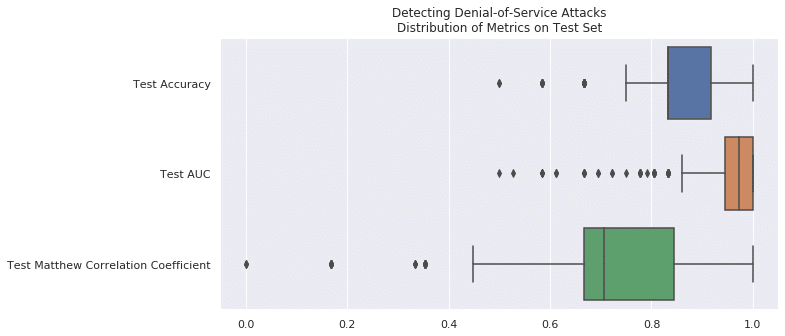
Results
We measure our model using accuracy, AUC, and Matthew Correlation Coefficient over 500 trials. Due to the even number of positive and negative example in the dataset, random chance is 0.500 for accuracy and AUC. Furthermore, there is no correlation between random prediction, so the Matthew Correlation Coefficient is 0.0. The results compare very favorably to a random chance.
| Accuracy on Test Set @ 500 Trials | AUC on Test Set @ 500 Trials | Matthew Correlation Coefficient on Test Set @ 500 Trials | |
| Chance | 0.5000 | 0.5000 | 0.0000 |
| Random Forest | 0.8632 ± 0.0974 | 0.9494 ± 0.0786 | 0.7495 ± 0.1833 |
Discussion
This is our initial attempt at detecting DDoS in an open, global, data source, and we achieved nominal success, but this isn’t the end goal though. We want to do this as soon as, or before, a DDoS begins. We believe this is possible due to the large spin-up time associated with organizing and communicating with the millions of devices/computers before an attack. This causes a large amount of network traffic, that should cause changes in BGP routing.
The challenging component of this analysis is the lack of data. To label the data used here, we combed numerous media reports, and we found that while reports will generally agree on the day (hence our analysis here), they will disagree on more specific times (if they report them at all). Fortunately, this is a hurdle that should ease with time, as vulnerable devices and attacks begin receiving detailed reports. We await that time. Happy hunting!