
Neural networks use a One-vs-All scheme to perform multinomial classification (using the highest response from K output neurons as the predicted class). The same general approach is used in classical machine learning techniques, with the same limitations. To get around these pitfalls, a range of alternative techniques were developed. This post takes a few of these alternatives (namely All-vs-All and a Hierarchical scheme) and applies these to neural network modeling, and deep learning in general.
Motivating Example
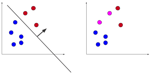
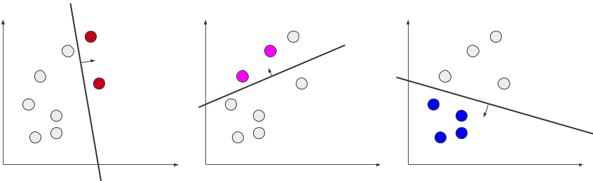
Consider that we want to separate two distinct classes. In this binary case, we can use a technique like Support Vector Machines (SVMs) to determine the hyperplane that best separates the classes. This separation isn’t as straight forward when dealing with more than two classes (done!). So, now imagine we have three classes to separate (a multinomial problem). A single hyperplane will not separate these points, so we need some alternative strategies. What we can do is take a single class and find the hyperplane that separates it from all other points. Doing this for each class, we now have three classifiers (hyperplanes). Serially applying the hyperplanes to a new point, we can classify based on which hyperplane produces the largest response (inner product). We have just performed One-vs-All classification (one of the most common techniques for classification).
There are two major problems with this approach. The first is that response values may differ between the classifiers and, more importantly, this scheme can become unbalanced when comparing a single class to all other points. For example: if there are 2 points in each of the 10 classes, then each binary classifier will compare 2 positive examples to 18 negative examples.
Multinomial Classification
The One-vs-All classification is not the only approach, though. One-vs-All produces a model for each class (number of classes = K). You can then compare a new point to each classifier.
All-vs-All by comparison, creates a classifier for every pair of classes (Comb(K,2) = K(K-1)/2). To determine the label of a new point, we now predict with each classifier and use some voting rule to determine the most likely class. This mitigates some of the balancing issues that One-vs-All might have.
Hierarchical methods are a more general set of approaches, where some organizational scheme is used to determine the class. You could imagine this method as whittling down the list of classes by removing the most unlikely label at each step. We classify this approach as tree-like based on how we apply it here. All classes are considered initially, then we choose a branch based on the least likely class (removing it from consideration). We continue branching in this way until we have only 1 class remaining, our prediction. This will require 2K trained models, but we will only traverse (predict) K-1 of them during prediction.
In general, if a multi-class machine learning (ML) method doesn’t specify, it’s probably One-vs-All.
Neural Network Classification
Neural Network (NN) models use a slightly different approach. While for binary classification a single output neuron is sufficient, this is not the case for multi-class problems. The standard approach is to have K output neurons, convert them to a probability distribution with a softmax activation, and take the highest response as the class. This is similar (although not equivalent) to the One-vs-All regime. There are K outputs that we are comparing. This begs the question of what would the other classification schemes look like under NNs.
Idea
Apply the All-vs-All and Hierarchical classification schemes to neural networks.
Advantages:
- Generally, these approaches should give increased performance.
Disadvantages:
- These methods require more compute and memory than One-vs-All.
The approach here will be to substitute the One-vs-All output layer for the layers necessary to approximate the All-vs-All and Hierarchical scheme.
All-vs-All:
- For this we will instantiate (K(K-1)/2) models where the output is a dense layer with 2 nodes for comparing 2 classes.
- The predicted class for a new point will then be chosen based on the highest cumulative response across all classes.
Hierarchical:
- We will instantiate 2K models where the output layer is every combination of the K classes (I know this is a lot!).
- The predicted class will be chosen by performing classification at each step and removing the class that has the lowest response.
- We continue until a pairwise comparison is made and the highest responding class is determined.
Computational Details
Assuming we used the same model architecture for the comparisons (and only switched the output layer), a naive implementation of this would require O[K(K-1)/2*M] bytes of storage in the All-vs-All case (where M is the number of bytes to store a single model). Because this would require O[2K*M] bytes to store the full model in the hierarchical case, let’s be a bit smarter about this. Instead, we train a single One-vs-All model (like normal) and use transfer learning, replacing the One-vs-All output layer with the output layer needed for the All-vs-All and Hierarchical methods. This reduces the storage requirements for All-vs-All and Hierarchical to O[M+K(K-1)/2] and O[M+2K] bytes respectively, and also reduces the training requirements. It’s worth noting that the All-vs-All and Hierarchical approaches are extremely parallelizable (although we save that implementation for a later post).
Evaluation
Well…let’s test it out. To do this we take some standard datasets and a standard model architecture and compare test accuracies. We will also sub-sample the data uniformly. This will hopefully accentuate the differences in the methods. Each experiment is run 10 times. Code is available here.
Datasets
We use two datasets for this evaluation: CIFAR-10 and MNIST. CIFAR-10 is a dataset of 50,000 RGB color images (shaped 32-by-32-by-3). MNIST is a dataset of 60,000 grayscale images (28-by-28-by-1). These datasets were chosen due to ease of access, my affinity towards images, and more importantly, the wealth of literature on good classification accuracies. The data is normalized to have pixel values in the range [0,1]. The preprocessing code is below. Lots of restrictions are taken for time/compute reasons.
import numpy as np
from keras.utils import to_categorical
from keras.datasets import mnist, cifar10, fashion_mnist

dataset = "mnist" # {"mnist", "cifar10", "fashion_mnist"}

# Load Data
if dataset == 'mnist':
    (x_train, y_train), (x_test, y_test) = mnist.load_data()
    labels = ['0','1','2','3','4','5','6','7','8','9']
elif dataset == 'cifar10':
    (x_train, y_train), (x_test, y_test) = cifar10.load_data()
    labels = ['airplane','automobile','bird','cat','deer','dog','frog','horse','ship','truck']
elif dataset == 'fashion_mnist':
    (x_train, y_train), (x_test, y_test) = fashion_mnist.load_data()
    labels = ['T-shirt/top','Trouser','Pullover','Dress','Coat','Sandal','Shirt','Sneaker','Bag','Ankle boot']
else:
    raise(ValueError(f"I don't know what {dataset} is!nChange to one of 'mnist', 'cifar10', or 'fashion_mnist'."))

# Normalize and Reshape Data
x_train_orig = x_train.astype('float32') / 255.
x_test_orig = x_test.astype('float32') / 255.

if dataset in ['mnist','fashion_mnist']:
    x_train_orig = x_train_orig.reshape(x_train_orig.shape + (1,))
    x_test_orig = x_test_orig.reshape(x_test_orig.shape + (1,))

# Encode Labels
y_train_list = y_train.ravel()
y_test_list = y_test.ravel()
y_train = to_categorical(y_train)
y_test = to_categorical(y_test)

# Restrict to Lower 5 Classes (for time reasons)
x_train_orig = x_train_orig[y_train_list < 5]
y_train = y_train[y_train_list < 5]
y_train_list = y_train_list[y_train_list < 5]
x_test_orig = x_test_orig[y_test_list < 5]
y_test = y_test[y_test_list < 5]
y_test_list = y_test_list[y_test_list < 5]

# Subsample Every 10 Training Examples (for time reasons)
x_train = np.array(x_train_orig)[::10,:,:,:]
x_test = np.array(x_test_orig)[::1,:,:,:]
y_train = y_train[::10,:]
y_test = y_test[::1,:]
y_train_list = y_train_list[::10]
y_test_list = y_test_list[::1]
Model
The network architecture is a simple convolutional network (LeNet):
- 32 convolution filters with a stride of 1 and a kernel size of 3-by-3
- 64 convolution filters with a stride of 1 and a kernel size of 3-by-3
- Max pooling layer for 2-by-2 pixel values
- Flatten layer
- Dropout layer 0-masking 25% of the pixels
- Fully connected layer with 256 neurons and a ReLU activation function
- Dropout layer 0-masking 50% of the pixels
- Fully connected layer with 10 neurons as the output layer with a softmax activation function
We change the output layer (as described above) for the All-vs-All and Hierarchical schemes. The model creation code is below:
import keras

def build_LeNet(shape):
    l1 = keras.Input(shape=shape)
    l2 = keras.layers.Conv2D(filters=32, kernel_size=(3,3), activation='relu')(l1)
    l2 = keras.layers.Conv2D(filters=64, kernel_size=(3,3), activation='relu')(l2)
    l2 = keras.layers.MaxPooling2D(pool_size=(2,2))(l2)
    l2 = keras.layers.Flatten()(l2)
    l2 = keras.layers.Dropout(.25)(l2)
    l2 = keras.layers.Dense(units=256, activation='relu')(l2)
    l2 = keras.layers.Dropout(.5)(l2)
    l2 = keras.layers.Dense(units=10, activation='softmax')(l2)
    return (l1, l2)
Experiment
There are a bunch of parameters that are all listed in the repository. We list the more relevant ones below:
- 12 epochs to train the base model
- 20 epochs to train any models related to All-vs-All and Hierarchical models
- 128 sample batch size
- Adadelta as the optimizer
Results
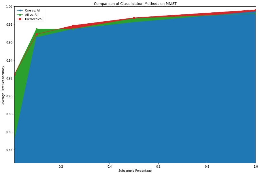
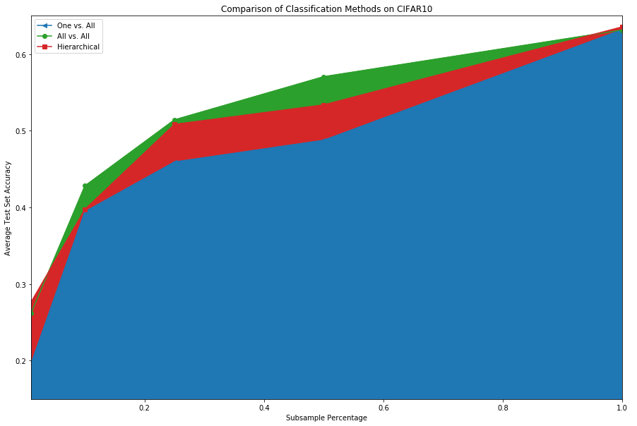
In summary, the alternative methods seem to add some value, especially when there are fewer training samples. For the MNIST dataset the deviations in the test accuracy were ~1E-16 (machine epsilon) over the 10 trials performed. The CIFAR10 dataset, on the other hand, had a p-value < 0.0001 and a normalized effect size (Cohen’s d) of 29.9 for the 1% subsample (and a non-significant result for the 100% subsample: p-value=.28, effect size=.25). See the table below for the numbers.
| MNIST | One-vs-All (mean ± std @ 10 trials) | All-vs-All | Hierarchical |
| 1% Subsample Test Accuracy | 0.85 ± 0.00 | 0.92 ± 0.00 | 0.92 ± 0.00 |
| 10% Subsample Test Accuracy | 0.96 ± 0.00 | 0.97 ± 0.00 | 0.96 ± 0.00 |
| 25% Subsample Test Accuracy | 0.97 ± 0.00 | 0.97 ± 0.00 | 0.97 ± 0.00 |
| 50% Subsample Test Accuracy | 0.98 ± 0.00 | 0.98 ± 0.00 | 0.98 ± 0.00 |
| 100% Subsample Test Accuracy | 0.99 ± 0.00 | 0.99 ± 0.00 | 0.99 ± 0.00 |
| CIFAR10 | |||
| 1% Subsample Test Accuracy | 0.19 ± 0.00 | 0.26 ± 00 | 0.27 ± 0.00 |
| 10% Subsample Test Accuracy | 0.39 ± 0.01 | 0.42 ± 04 | 0.39 ± 0.02 |
| 25% Subsample Test Accuracy | 0.45 ± 0.04 | 0.51 ± 02 | 0.50 ± 0.01 |
| 50% Subsample Test Accuracy | 0.48 ± 0.03 | 0.57 ± 00 | 0.53 ± 0.01 |
| 100% Subsample Test Accuracy | 0.63 ± 0.01 | 0.63 ± 00 | 0.63 ± 0.00 |
Future Work
There are a lot of interesting questions this work brings up. I didn’t have time to explore them, but possibly will in a future blog post.
- Would training the All-vs-All and Hierarchical models from scratch produce different results?
- To some extent, this must be the case and replacing the output layer produced different results, but maybe training from scratch converges to a much different set of weights.
- What is the mechanism causing major differences in the models when there are few training examples?
- I imagine it might have to do with the class imbalance.
- Could the Hierarchical model be modified to remove more than 1 class at each step?
- It’s certainly the case that there are examples where the top choice doesn’t change after removing low probability classes.
- How often does this occur, and how much compute can be saved?


Bridging the gap between the impossible and the practical with innovative technology solutions in cyber, data science, mobile, microelectronics and information operations and a full spectrum of products and capabilities to advance national security missions.