
What is alert merging?
Extended cyber attacks are complex things, reaching across time and alerts. To understand the full scope and impact of such an attack, analysts will need to consider multiple alerts in concert. However, it might not be obvious which alerts are related to each other, and which are not. Here we discuss using machine learning to implement alert merging, which strives to identify those alerts that are related to each other.
There are other tools that already attempt this task, such as entity matching in The Hive, which can report on alerts that share a common entity. Our goal is something more than this, though, in several aspects:
- Provide a score indicating how related alerts are, rather than simply stating “these alerts share an entity”
- Parse and directly compare alerts from different detectors and in varying formats
- Detect cases where entities are similar, but not exact matches (similar timestamps, related adversary tactics, techniques, and procedures (TTPs), etc.)
This won’t be relevant in all contexts. We’re thinking about SOC (Security Operations Center) -type situations, where analysts quickly (sometimes extremely quickly) analyze alerts from many detectors. They may not have the time or bandwidth to consider which non-obviously related alerts they should considered together. We’re trying to analyze already existing alerts, and improve the context in which analysts consider cyber events.
The Machine Learning model
We’re using a neural network to classify the relationship between pairs of alerts. Autokeras’ Automodel selects and trains the specific layers of the network to produce a classifier that detects whether two alerts are related or not.
In detail
Selecting network features from cyber data is hard, especially when using data from multiple sources. Relevant fields differ; timestamps are in varying formats; different alerts focus on different adversarial activities and indicators. We’ve made the model less dependent on these specifics by concatenating fields within log lines and turning them all into strings when training. This neatly side-steps the entire issue of feature selection: Autokeras itself will vectorize the string and pick out the relevant features. This also bypasses other issues like “How do you parse an IP address,” and ensuring that all timestamps are in the same format.
Creating labels is straightforward: we use training data labeled with the identity of the source cyber attack, and the ML labels are just “same” or “different” based on the attack labels of the two paired log lines.
The next step is training, which in our case just consists of letting Autokeras’ Automodel do its thing. We do have to select parameters like number of epochs and trials. In our case, we have a relatively small set of training data, so both of these values are fairly small. The result is a model trained to classify whether a pair of log lines resulted from the same cyber attack.
Data/Testing
Magicwand
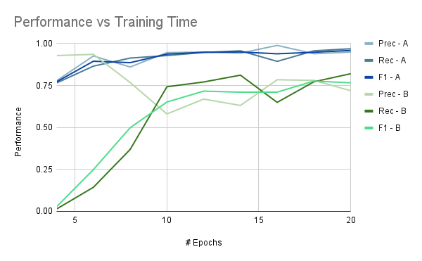
Before we tried this out on real-world data, we tested the idea out on more readily available (and more customizable) data. For this, we used Magicwand, a DDOS cyber attack data generation tool. We generated data from several cyber attacks, and ran tests to determine if we could train a model that would distinguish between log lines from different attacks. Since this is generated data, and not something collected in the wild, we modified some of the less-realistic artifacts (completely non-overlapping timestamps and distinct IP addresses, for instance) before training. And the model was successful! With fairly short training times (i.e. few epochs), we could achieve satisfactory results (F1 above .75) with all the subsets of the data we tried.
Real-world alerts
And now, the whole reason why we’re doing this work! The idea is that this model will run against threat detectors from other threat detection analytics. This will enhance the results both within a given threat detector, and also across multiple different ones.
The data format here is slightly different. Instead of individual log lines, we’re dealing with entire cyber alerts, often summarizing activity from a given detector for an entire day. This requires some modification to our design. Instead of log lines, we parse STIX data into “log-line equivalents” by using relationship objects to associate entities (IP addresses, users, host names, etc.). This causes each alert to be broken into multiple log lines (something in the 3-30 range, depending on the STIX data), which requires some modification of the algorithm: (1) the splitting of the data as described earlier, and (2) aggregation of the scores to form an overall score for the alert as a whole.
For training data, we used alerts from two red team events on a real enterprise network. These data provide the related alerts, and various other unrelated alerts fill out our dataset.
To predict on other stories, we run all pairwise log line comparisons between the two alerts in question through our model, and then aggregate the resulting scores (in this case, a simple average) to get a final score that represents the two alerts’ similarity. We ran various experiments to determine exactly the pairing required to get reliable performance. Using each log line once is not sufficient–we needed to do pairwise comparisons on all log lines from both alerts. My theory on the requirement for all comparisons: some events detailed in the STIX data are significantly more related and relevant to each other. If we happen to randomly pair up these related fragments, we get a very high score! If, however, we happen to miss those pairs, we’ll get an unrealistically low score. Using all pairwise comparisons ensures we don’t accidentally miss relevant pairs.
Results
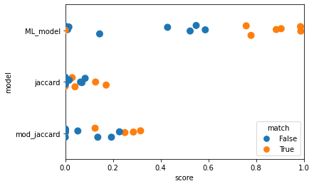
To assess our model, we compared it to two baselines.
- Jaccard similarity on the sets of entities in the two alerts
- Modified Jaccard similarity. We compute this as the size of the intersection of the two entity sets divided by the size of the smallest set. This gives a higher and more useful score in cases where one alert has much fewer entities but overlaps almost entirely with the other alert.
As this is a threshold-based model, we’re really looking for separation of the matching and differing stories. In Fig. 2.1, we certainly see more separation with the machine learning model than with either the standard Jaccard similarity, or the modified Jaccard similarity.
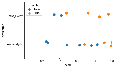
Another important consideration: what happens if there is a new attack, or if a new analytic is added? Will the model need to be retrained? For a new attack, we definitely do not want to have to retrain the model. That would, more or less, defeat the purpose of the entire thing. We want our model to detect and match new attacks on its own. In the case of a new analytic, retraining is less of a problem. Adding new analytics happens relatively infrequently, and retraining therefore won’t be entirely prohibitive.
We ran experiments to simulate these situations, shown in Fig. 2.2. We trained the model using a specific subset of our data, selected for each experiment. To simulate a new attack, we trained using data from only one red team event. To simulate a new analytic, we used data only from one of our two analytics. We then tested these models using the data we held out (the other event and other analytic, respectively). The separation we want is still fairly apparent with a new event, although less so with a new analytic. This is what we were aiming for, and shows this model can be expected to detect new events. New analytics, however, will benefit from retraining.
Interesting lessons
Shuffling the order of the log line fields during stringification improves performance. This could be because it makes the model less reliant on specific formats or orders. Instead, the model learn things about the events themselves (e.g. proximity in time, similarity of the TTPs, similarity of the IPs, etc.).
Further work
We talked to a cyber analyst, who had suggestions on what would make this more useful. For instance, he uses a lot of other data not listed in log lines or alerts. One example he’d like to see included is a check on how new a domain name is. If it’s really new, that would be a big red flag! If it’s well established, the activity is less likely to be malicious and interesting.
This is machine learning, so wanting more data is practically a tautology. Training on more red team events will help us understand whether further events allow the algorithm to learn about different attacker strategies, or if there is some typical through-line in this sort of event that the model will latch onto. We can also examine how the model behaves when used on a new platform. How necessary is retraining? Will results on a new platform have any meaning, or will the output be a huge pile of random numbers?
This effort could also be expanded into full-blown campaign detection by incorporating additional features, like the newness of a domain name. Rather than simply predicting whether two past alerts are related to each other, it could be retrained to detect and create alerts about ongoing cyber attacks.
Machine learning in cyber security is an area with many possibilities for research and advancement, and one in which there are lots of efforts taking place. There are a lot of possible applications for this sort of work, both in repurposing existing machine learning strategies to work with cyber security data, and in developing new strategies. This post is just a brief jaunt into one of the many possible applications.
This research was developed with funding from the Defense Advanced Research Projects Agency (DARPA).
The views, opinions and/or findings expressed are those of the author and should not be interpreted as representing the official views or policies of the Department of Defense or the U.S. Government.
Distribution Statement “A” (Approved for Public Release, Distribution Unlimited).